Masking Strategies for Background Bias Removal in Computer Vision Models

ICCV 2023 Workshops (OOD-CV) · Paris, France
1Inria · 2INRAE · 3University of Montpellier · 4LIRMM · 5UMR-TETIS
*Corresponding Author: ananthu.aniraj@inria.fr

Background Bias in Fine-Grained Classification

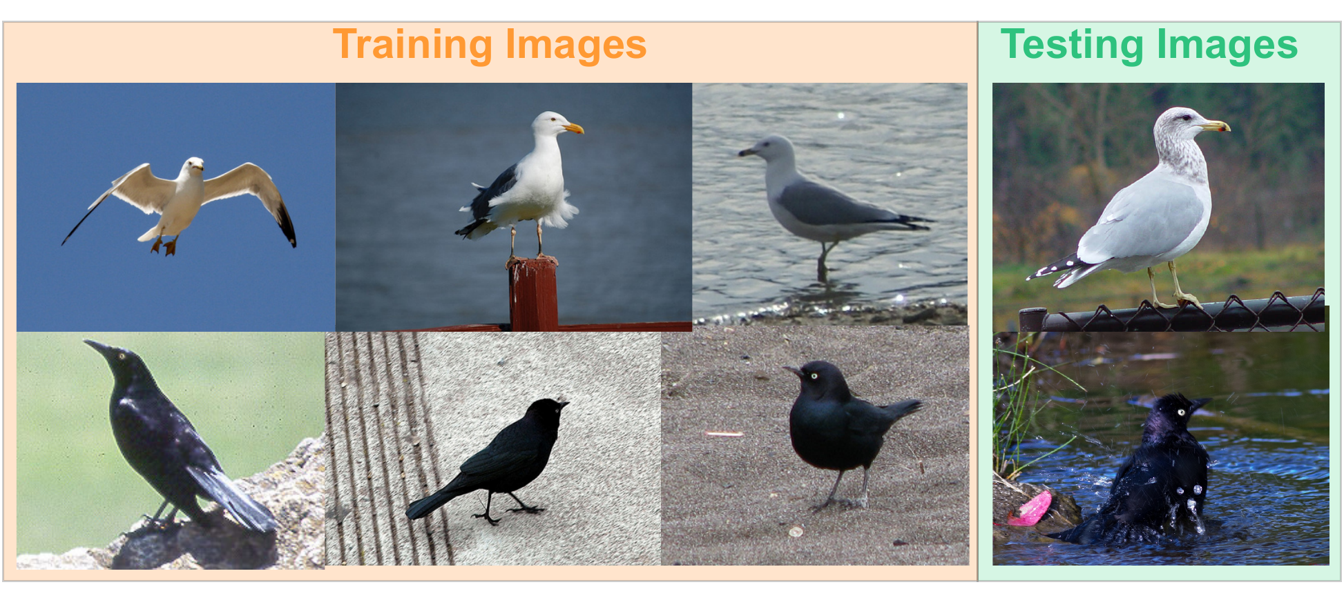
Background bias in fine-grained bird species classification: standard models rely on habitat background cues
Figure 1: Background bias in fine-grained classification. Computer vision models trained on object-centric tasks (such as fine-grained bird species classification in CUB-200-2011) inadvertently learn spurious correlations between species and their typical habitat backgrounds (e.g. waterbirds appearing on water). When tested in real-world scenarios on Out-of-Distribution (OOD) backgrounds (e.g. waterbirds appearing in a bamboo forest from Places365), standard deep models suffer drastic accuracy drops due to shortcut learning.
🎯
Subtle Distinctions
Fine-grained categories share almost identical visual traits, making models prone to relying on external habitat shortcuts.
🌲
Spurious Correlations
Strong co-occurrence between bird species and environmental backgrounds leads models to classify the scene rather than the animal.
📉
Severe OOD Degradation
Deploying on novel environments causes baseline models to drop up to 30% in Top-1 accuracy when the background changes.

Abstract

Models for fine-grained image classification tasks, where the difference between some classes can be extremely subtle and the number of samples per class tends to be low, are particularly prone to picking up background-related biases and demand robust methods to handle potential examples with out-of-distribution (OOD) backgrounds.

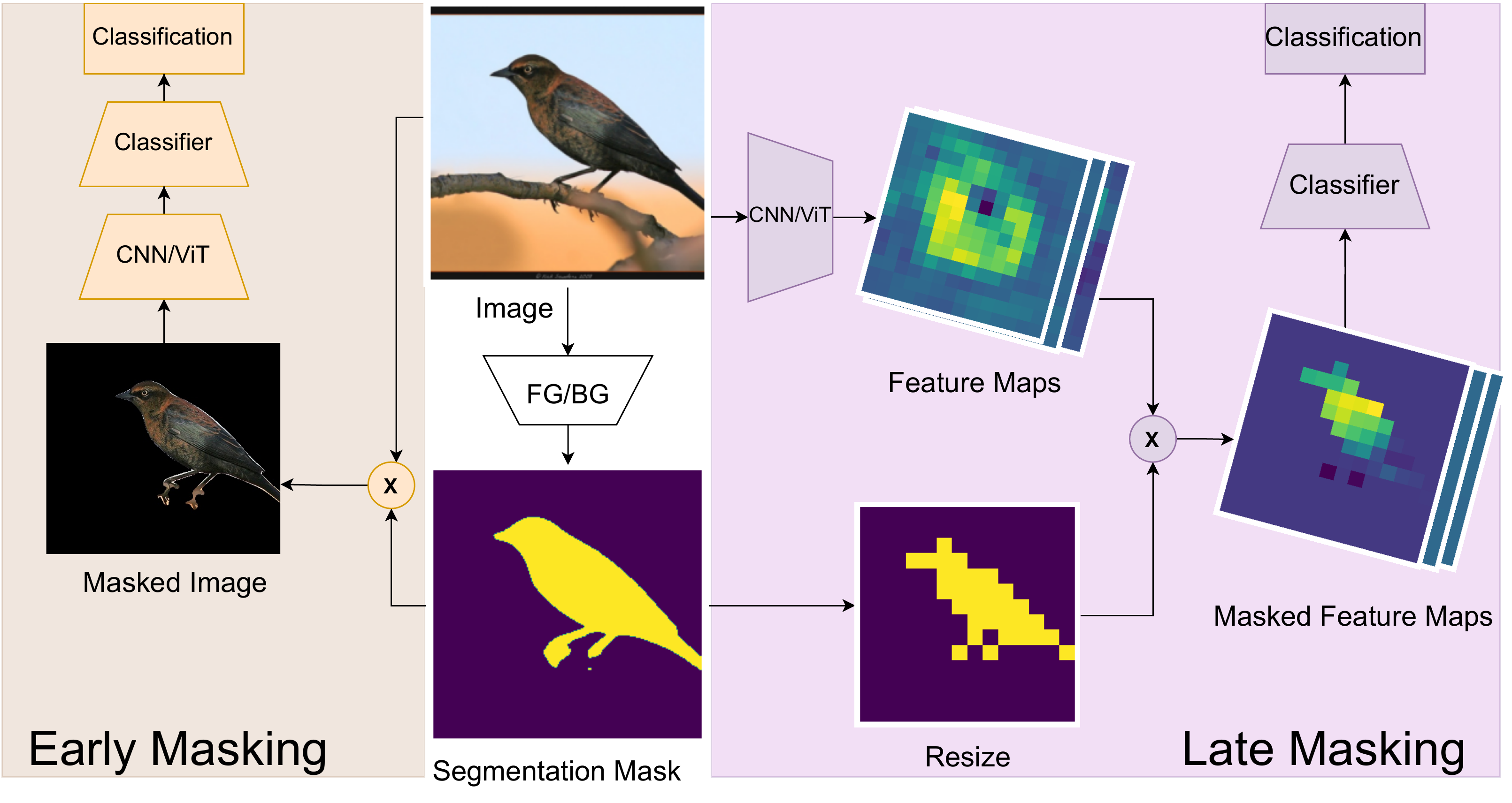
To gain deeper insights into this critical problem, our research investigates the impact of background-induced bias on fine-grained image classification, evaluating standard backbone models such as Convolutional Neural Networks (CNNs) and Vision Transformers (ViTs). We explore two masking strategies to mitigate background-induced bias: Early masking, which removes background information at the (input) image level, and late masking, which selectively masks high-level spatial features corresponding to the background.

Extensive experiments assess the behavior of CNN and ViT models under different masking strategies, with a focus on their generalization to OOD backgrounds. The obtained findings demonstrate that both proposed strategies enhance OOD performance compared to baseline models, with early masking consistently exhibiting the best OOD performance. Notably, a ViT variant employing GAP-Pooled Patch token-based classification combined with early masking achieves the highest OOD robustness.
Masking Strategies

Early and late masking strategies for background bias removal
Figure 2: Overview of the proposed Early and Late Masking strategies. (Left) Early Masking: The binary foreground mask is applied directly at the input image stage, filtering out all background pixels before feature extraction. (Right) Late Masking: The full image is processed through the backbone, and background-related high-level spatial features are selectively masked out prior to the classification head.
Early Masking (EM)

Masking at the input image stage ($L = 0$). Background pixels are suppressed prior to entering the backbone:

$$\mathbf{y} = g_{\theta_2}\big(h_{\theta_1}(\mathbf{x} \odot \mathbf{m})\big)$$
  • $\mathbf{x} \in \mathbb{R}^{3 \times M \times N}$: Input RGB image.
  • $\mathbf{m} \in \{0, 1\}^{1 \times M \times N}$: Binary foreground mask predicted by a pre-trained Mask2Former network.
  • $h_{\theta_1}(\cdot)$: Classification backbone (ConvNeXt or DINOv2 ViT).
  • $g_{\theta_2}(\cdot)$: Classification head producing logits $\mathbf{y} \in \mathbb{R}^C$.
  • Advantage: Eliminates background shortcuts at the source, preventing spurious contextual representations from forming in both CNNs and ViTs.
Late Masking (LM)

Masking high-level spatial representations inside the network ($L > 0$):

$$\mathbf{y} = g_{\theta_2}\big(h_{\theta_1}(\mathbf{x}) \odot \mathbf{m}'\big)$$
  • $\mathbf{z} = h_{\theta_1}(\mathbf{x}) \in \mathbb{R}^{D \times M' \times N'}$: Spatial feature tensor output by the backbone ($M' = M/k$, $N' = N/k$).
  • $\mathbf{m}' \in \{0, 1\}^{1 \times M' \times N'}$: Downsampled binary foreground mask matching feature resolution.
  • $g_{\theta_2}(\cdot)$: Global average pooling (GAP) followed by linear classification layer.
  • Advantage: Allows low-level layers to exploit natural image gradients while explicitly removing background activations from the final decision layer.

Binary Semantic Foreground-Background Segmentation

To obtain the binary foreground mask $\mathbf{m}$, we fine-tune a pre-trained Mask2Former model with a Swin-Tiny backbone on CUB-200-2011 segmentations. The model generalizes exceptionally well, achieving a Mean Dice score of 96.05% on CUB bird foregrounds and 91.84% on out-of-distribution Waterbirds images without any OOD retraining.

Experimental Evaluation

All models are trained exclusively on CUB-200-2011 (200 bird species, 5,994 train images) and evaluated on both In-Distribution (CUB test) and Out-Of-Distribution adversarial backgrounds (Waterbirds, 5,794 images on Places365 backgrounds).

Model Training Setting CUB Test (In-Distribution) Waterbirds Test (Out-of-Distribution)
Original Test Masked Test Original Test Masked Test
ConvNeXt-S Baseline 86.56% 78.60% 55.82% 67.12%
Early-Masked 83.84% 84.43% 64.21% +8.39% 77.33% +10.21%
ConvNeXt-B Baseline 88.00% 77.52% 65.96% 68.51%
Early-Masked 84.36% 85.69% 67.21% +1.25% 80.10% +11.59%
ConvNeXt-L Baseline 88.05% 78.68% 66.83% 70.69%
Early-Masked 87.22% 87.38% 73.67% +6.84% 82.81% +12.12%
ViT-S Baseline 88.26% 82.27% 71.15% 77.59%
Early-Masked 85.89% 87.92% 78.61% +7.46% 84.05% +6.46%
ViT-B Baseline 89.20% 87.69% 76.65% 83.00%
Early-Masked 88.35% 90.10% 82.15% +5.50% 86.93% +3.93%
ViT-L Baseline 89.79% 88.91% 80.76% 85.61%
Early-Masked 88.35% 91.06% 84.67% +3.91% 88.30% +2.69%

Key Takeaway: Across all model scales (Small, Base, Large) and architectures (ConvNeXt & ViT), Early Masking consistently outperforms the baseline on OOD Waterbirds. For ViT-B and ViT-L, early masking also achieves the absolute highest in-distribution accuracy on CUB (90.10% and 91.06%), showing that ViTs are less sensitive to masking boundaries while benefiting from spurious background removal.

Backbone Strategy CUB Test (In-Distribution) Waterbirds Test (Out-of-Distribution)
Frozen Backbone Fine-tuned Frozen Backbone Fine-tuned
ConvNeXt-B Baseline 88.00% 89.62% 65.96% 76.20%
Early-Masked 85.69% 90.31% 80.10% 87.01% +10.81%
Late-Masked 87.66% 88.76% 77.95% 78.42%
ViT-B Baseline 89.20% 89.38% 76.55% 68.36% -8.19%
Early-Masked 90.10% 91.37% 86.93% 88.81% +20.45%
Late-Masked 88.61% 90.73% 76.55% 74.76% -1.79%

Critical Finding on Fine-Tuning: Fine-tuning the baseline ViT-B without masking causes severe overfitting to background correlations, dropping OOD Waterbirds accuracy from 76.55% down to 68.36% (-8.19%). In sharp contrast, Early Masking completely protects the ViT, boosting its OOD accuracy to 88.81% (+20.45% over fine-tuned baseline) while achieving the highest in-distribution score (91.37%).

Backbone Feature Masking Stage CUB Test (%) Waterbirds OOD (%) OOD Relative Improvement
ConvNeXt-S Stage $L$ (Last Stage) 88.73% 77.19% Baseline LM
Stage $L-1$ (Second-to-Last) 89.35% 81.22% +4.03%
Stage $0$ (Input Image / Early) 90.73% 87.95% +10.76%
ConvNeXt-B Stage $L$ (Last Stage) 88.76% 78.42% Baseline LM
Stage $L-1$ (Second-to-Last) 89.04% 80.04% +1.62%
Stage $0$ (Input Image / Early) 90.31% 87.01% +8.59%
ConvNeXt-L Stage $L$ (Last Stage) 89.80% 79.39% Baseline LM
Stage $L-1$ (Second-to-Last) 89.49% 79.68% +0.29%
Stage $0$ (Input Image / Early) 90.99% 88.19% +8.80%

Receptive Field Analysis: Moving the masking stage earlier in the network ($L \to L-1 \to 0$) yields monotonic accuracy gains on both CUB and Waterbirds. Earlier CNN layers feature tighter, strictly localized receptive fields that correlate directly with image patches, whereas deeper layers blend background context into foreground feature channels.

Backbone Strategy ViT Representation CUB Test (In-Distribution) Waterbirds Test (Out-of-Distribution)
Frozen Fine-tuned Frozen Fine-tuned
ViT-B Baseline CLS Token 90.04% 90.47% 80.35% 71.35%
GAP-Pooled Patch 62.24% 90.05% 24.71% 67.74%
CLS + Patch 89.20% 89.38% 76.65% 68.36%
Early-Masked CLS Token 90.33% 91.73% 86.81% 88.60%
GAP-Pooled Patch 72.17% 91.51% 66.37% 89.22% Highest OOD
CLS + Patch 90.10% 91.37% 86.93% 88.81%
Late-Masked CLS Token 89.16% 90.78% 75.10% 80.54%
GAP-Pooled Patch 84.15% 90.85% 71.63% 84.50%
CLS + Patch 88.61% 90.73% 76.55% 74.76%

ViT Token Insights: The ViT variant utilizing Global Average Pooled (GAP) Patch tokens combined with Early Masking achieves the absolute highest OOD robustness (89.22%) of all evaluated configurations. Because patch tokens preserve explicit spatial locality, masking at the input forces every patch token to encode pure foreground characteristics, eliminating global shortcut cues that bleed into the standard CLS token.

Segmentation Model Backbone CUB-200-2011 Mean Dice (%) Waterbirds OOD Mean Dice (%)
Background Bird Foreground Background Bird Foreground
Mask2Former Swin-T (Selected) 99.42% 96.05% 98.74% 91.84%
Mask2Former ResNet-50 99.43% 96.12% 98.72% 91.81%

Segmentation Robustness: Fine-tuned Mask2Former with Swin-Tiny backbone achieves >96% Dice on in-distribution CUB birds and maintains 91.84% Dice on OOD Waterbirds without seeing a single Waterbirds or Places365 image during training.

Key Findings & Takeaways

🥇
1. Early Masking Dominates OOD Robustness
Masking at the input image level ($L=0$) consistently delivers the highest generalization across both CNNs and ViTs. By removing background pixels before feature extraction, early masking prevents spurious contextual correlations from ever being encoded.
⚠️
2. Fine-Tuning ViTs Requires Background Masking
When fine-tuned end-to-end without masking, ViTs severely overfit to background cues, experiencing an 8.2% drop in OOD accuracy. Early masking completely reverses this, enabling fine-tuning to reach peak OOD accuracy of 88.8% – 89.2%.
🧩
3. GAP-Pooled Patch Tokens Outperform CLS Tokens
Classifying via Global Average Pooled (GAP) patch tokens instead of the standard CLS token yields the strongest OOD model (89.22% on Waterbirds). Patch tokens enforce spatial locality, preventing contextual leakage into global representations.
📶
4. Earlier CNN Masking Stages Yield Strictly Better Results
In ConvNeXt models, moving feature masking from the last stage ($L$) to the second-to-last ($L-1$) and finally to the input image ($0$) produces monotonic OOD accuracy improvements ($77.2\% \to 81.2\% \to 88.0\%$) due to smaller, unpolluted receptive fields.

Code & Pre-trained Models

Our implementation supports both Early Masking and Late Feature Masking across ConvNeXt (Small/Base/Large) and DINOv2 Vision Transformers (Small/Base/Large), along with the complete pipeline for binary foreground segmentation using MMSegmentation.

# Early Masking: Masking at the input image level
# Code path: early_masking_and_baseline/fine_tune_dinov2.py

import torch
from torchvision import transforms

def apply_early_masking(image, binary_mask):
    """
    image: [B, 3, H, W] normalized input tensor
    binary_mask: [B, 1, H, W] binary mask where 1=foreground, 0=background
    """
    # Element-wise product suppresses all background pixels
    masked_image = image * binary_mask
    return masked_image

# Forward pass through backbone and classification head
# y = g_theta2( h_theta1( x * m ) )
masked_inputs = apply_early_masking(inputs, masks)
outputs = model(masked_inputs)
# Late Masking: Masking high-level spatial feature representations
# Code path: feature_masking/layers/fm_net_dinov2.py

import torch
import torch.nn as nn
import torch.nn.functional as F

class LateMaskedViT(nn.Module):
    def __init__(self, backbone, num_classes=200):
        super().__init__()
        self.backbone = backbone
        self.classifier = nn.Linear(backbone.embed_dim, num_classes)

    def forward(self, x, mask):
        # Extract spatial patch tokens [B, D, H', W']
        spatial_features = self.backbone.get_intermediate_layers(x)[0]
        
        # Downsample binary mask to spatial feature resolution
        mask_downsampled = F.interpolate(mask, size=spatial_features.shape[-2:], mode='nearest')
        
        # Apply late feature masking: y = g( z * m' )
        masked_features = spatial_features * mask_downsampled
        
        # GAP-pooled patch token classification
        pooled = masked_features.mean(dim=[-2, -1])
        logits = self.classifier(pooled)
        return logits
# Download pre-trained Mask2Former Swin-T checkpoint for CUB foreground extraction:
# https://github.com/ananthu-aniraj/masking_strategies_bias_removal/releases/download/model_release/mask2former_swint_iter_160000.pth

# Generate binary masked CUB dataset using MMSegmentation:
python mmsegmentation/gen_masked_image_dataset.py \
    --config mmsegmentation/configs/mask2former/mask2former_swin-t_cub.py \
    --checkpoint checkpoints/mask2former_swint_iter_160000.pth \
    --input_dir data/CUB_200_2011/images \
    --output_dir data/cub_binary_masked

BibTeX

@InProceedings{Aniraj_2023_ICCV,
    author    = {Aniraj, Ananthu and Dantas, Cassio F. and Ienco, Dino and Marcos, Diego},
    title     = {Masking Strategies for Background Bias Removal in Computer Vision Models},
    booktitle = {Proceedings of the IEEE/CVF International Conference on Computer Vision (ICCV) Workshops},
    month     = {October},
    year      = {2023},
    pages     = {4397-4405}
}